GDAP session workflow

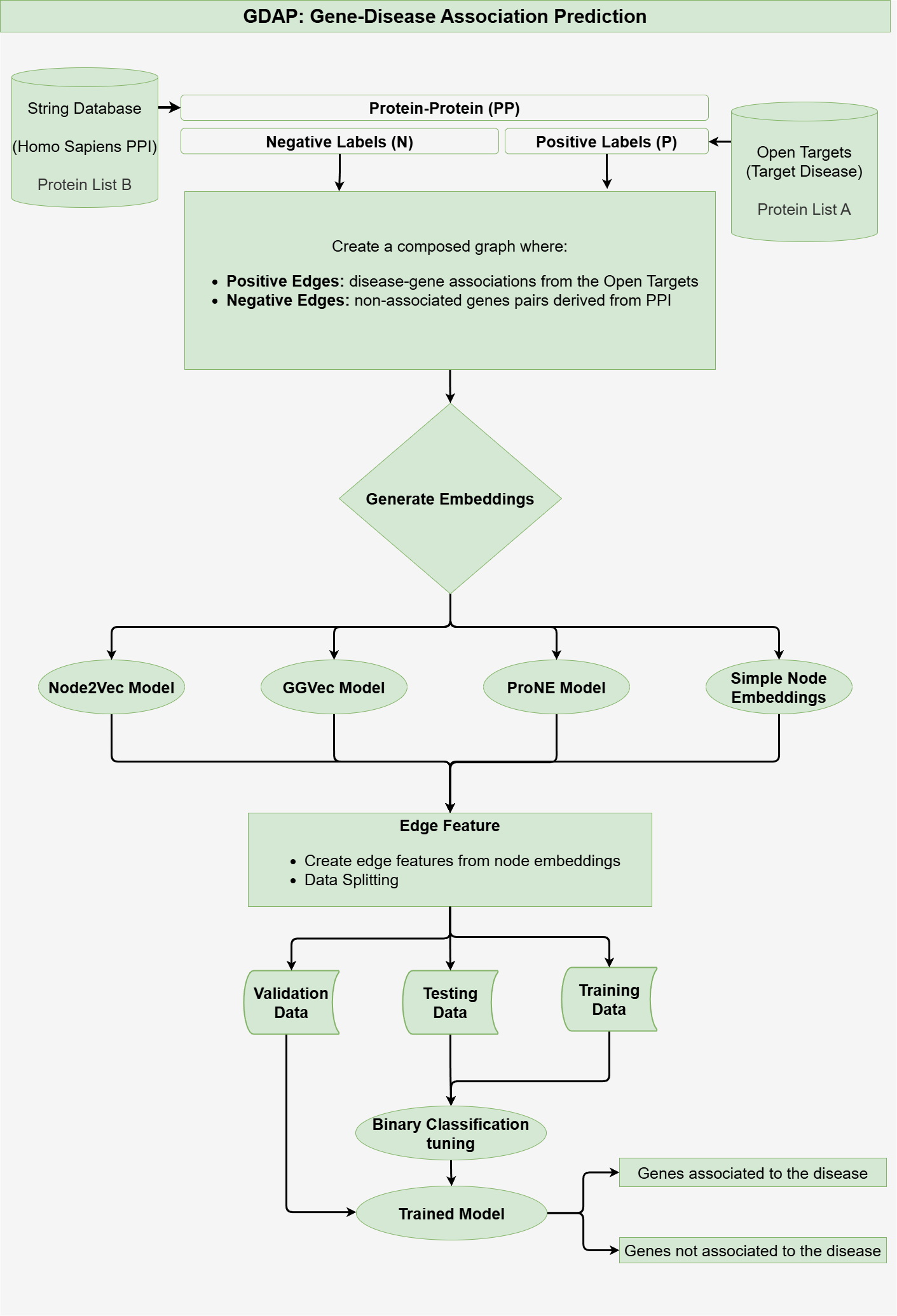
The GDAP workflow predicts gene-disease associations by leveraging disease-gene association data and Protein-Protein Interaction (PPI) data.

The GDAP workflow comprises three primary steps:

1. Data Collection: Fetching disease-gene and PPI data.
2. Graph Construction: Building a graph that integrates disease-gene and PPI data.
3. Embedding Generation: Using embedding models to represent graph nodes for prediction tasks.
4. Feature Extraction: Extract edge features, and split the data.
5. Model Selection: Training the model and generating predictions based on the features.

1. Data Collection

The first step in the GDAP workflow involves gathering the necessary data from two critical datasets:

1.1 Open Targets Dataset

The Open Targets platform provides a comprehensive resource for identifying therapeutic drug targets, offering data on disease-gene associations. GDAP utilizes two primary methods for accessing this data: the GraphQL API and Google BigQuery. Both methods offer different approaches for querying disease-target association data which are identified by Experimental Factor Ontology (EFO) terms.

Data Sources:

(i) GraphQL API:

• The GraphQL API enables you to retrieve disease-target association data using a flexible GraphQL querying structure. You can interact with the Open Targets GraphQL schema, which allows you to request detailed information about diseases and their associated targets, along with scores and other relevant metrics using the disease’s experimental variable.

  GraphQLClient Endpoints and Queries

  • GraphQLClient interacts with the Open Targets GraphQL Schema to fetch disease-target association data.
  • According to the Open Targets community forum, when using the GraphQL API, you need to iterate through each page of the disease to retrieve the overall results, as their API provides 50 results for each query. This is also outlined in their webinar.
  • The GraphQLClient first fetches the total number of targets associated with a specific disease using its EFO ID. This provides the necessary data to calculate how many pages of results need to be retrieved. Then, it iterates through each page, retrieving detailed disease-target association data, including target symbols and scores, until all results are collected.
  • In summary, the class performs the following steps:
    • 1. Retrieves the total count of targets associated with the disease.
    • 2. Iterates through all pages of results, collecting the complete dataset.
  • You can also run GraphQL queries through the GraphQL API Playground to explore or customize your queries.

(ii) Google BigQuery:

• Google BigQuery offers asynchronous SQL querying capabilities through Google Cloud’s infrastructure, providing an alternative method for extracting disease-target data.

  BigQueryClient Endpoints and Queries

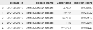
  • The BigQueryClient class allows you to query disease-target association data using Google BigQuery. It supports two main SQL queries: DIRECT_SCORES and INDIRECT_SCORES, which can be executed against the Open Targets BigQuery database.
    • DIRECT_SCORES: Retrieves the direct associations between diseases and targets, along with relevant scores and evidence counts.
    • INDIRECT_SCORES: Retrieves the indirect associations between diseases and targets, with corresponding scores and evidence counts.
  • You can also use these SQL queries directly in the BigQuery console for your specific disease and download the dataset in formats like CSV or JSON. Access the console.

1.2 String Database

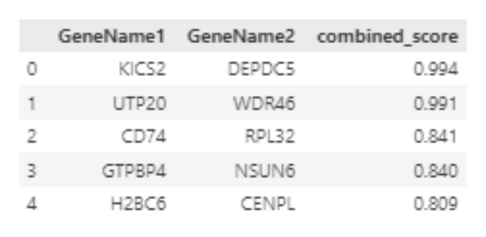
The STRING database provides a comprehensive network of protein-protein interactions (PPIs) for Homo sapiens. Each interaction is assigned a combined score, a probabilistic measure derived from multiple evidence sources, such as experimental data and text mining. This score quantifies the likelihood of interaction, forming the backbone for integrating disease-gene data with protein interactions in the GDAP workflow.

2. Graph Construction

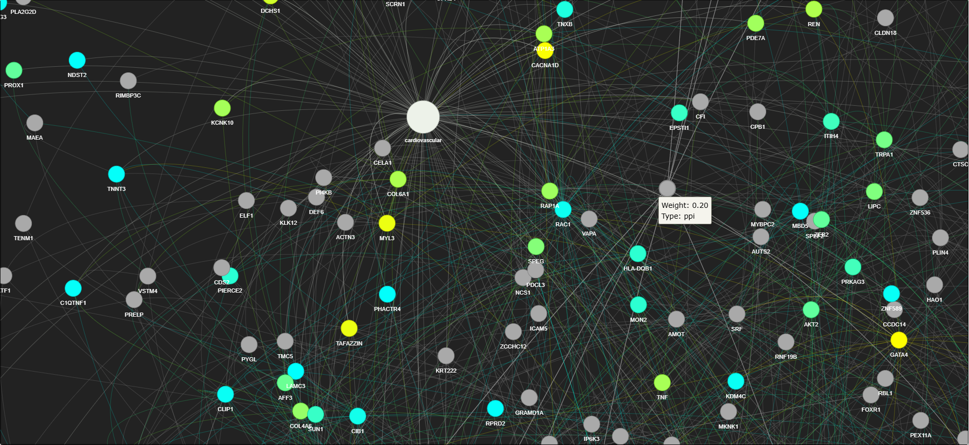
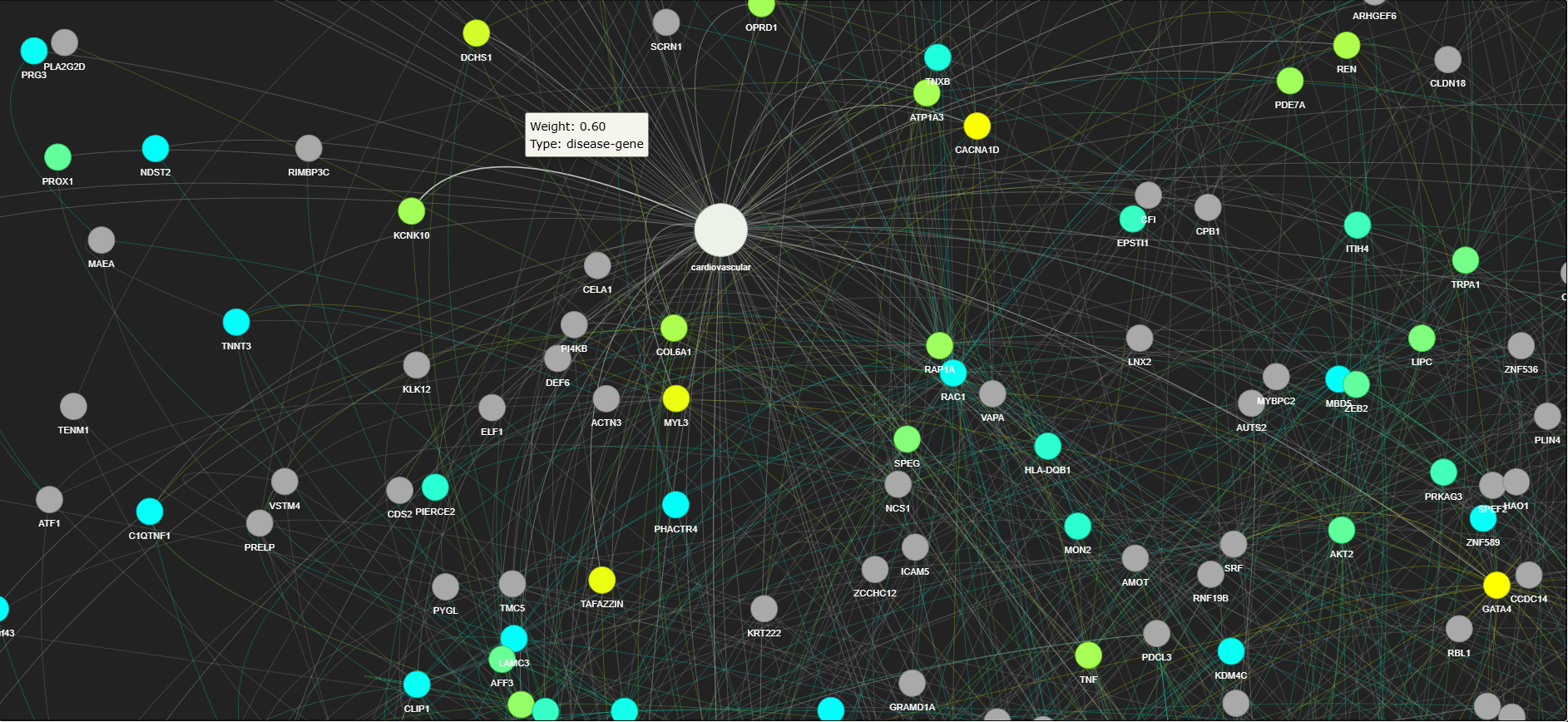
The graph construction step forms the core of the GDAP pipeline. It integrates both disease-gene associations and protein-protein interactions to form a bipartite graph.

This stage integrates the disease-gene associations and PPI data into a bipartite graph:

• Nodes: Represent the target (disease), and the genes (proteins).

• Edges: Represent relationships between nodes.

  • Positive edges represent disease-gene associations (edges weighted by their relevance scores from Open Targets).
  • Negative edges represent non-associated gene pairs, weighted by their interaction combined scores from the STRING database.

• The goal here is to construct a network that connects disease to genes and represents their biological relationships, along with possible interactions between genes.

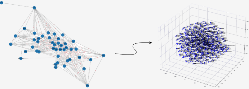
3. Embedding Generation

Node embeddings are generated using various nodevectors models to represent graph nodes in a lower-dimensional space.

These embeddings capture the structural and relational properties of nodes within the graph, ensuring that nodes representing similar biological entities or interactions are closely aligned in the vector space, which facilitates accurate predictions.

4. Feature Extraction and Data Splitting

Edge features are generated by combining the embeddings of the two nodes connected by each edge, capturing the relationship between them.

• For each edge, the embeddings of the connected nodes (disease and gene) are retrieved.
• The edge feature is created by multiplying these embeddings, resulting in a feature vector representing the relationship.
• The data is then split into training, validation, and testing sets: the training set is used for model fitting, the validation set for hyperparameter tuning, and the testing set to evaluate the model’s generalizability.

These edge features, derived from node embeddings, are essential for capturing relationships like disease-gene or protein-protein interactions. They are used to train a machine learning model for tasks such as predicting novel disease-gene associations or interactions.

5. Model Selection

The final step involves training a binary classifier to predict disease-gene associations. Currently, GDAP offers traditional machine learning algorithms and a simple dense sequential model.

(i) Model Training:

• Binary Classification: The classifier is trained using edge features. Positive edges (true associations) are labeled as 1, while negative edges (random or non-associating gene pairs) are labeled as 0.
• During training, the classifier learns to distinguish between true disease-gene associations and random connections, based on features derived from node embeddings and interaction strengths.

(ii) Model Prediction:

• After training, the model can predict new disease-gene associations or protein interactions by applying the learned model to novel edge pairs. The output is a probability score representing the likelihood that an edge (disease-gene or protein-protein interaction) is real.
• A threshold is applied to this score to decide whether the predicted edge is a positive or negative association (default threshold = 0.5).

(iii) Model Evaluation:

• The model’s performance is evaluated using metrics such as accuracy, precision, recall, and F1 score. These metrics assess how well the model generalizes to unseen data, ensuring that the predictions are meaningful and reliable.