
Introduction
In this notebook, we explore the creation and analysis of disease-gene and protein-protein interaction networks using the NetworkX library. We will fetch relevant datasets, construct directed and undirected graphs, and visualize disease-specific networks, with a focus on breast cancer and other diseases. By the end, we will have a comprehensive understanding of network creation and analysis methods applicable to various diseases from open target platform.
![]()
Table of Contents
- Fetching Datasets
- Graph Creation and Visualization with NetworkX
- Disease-Specific Graph Construction
- Integrating Graphs and Class Definitions
We need to get the Open Targets disease data and then get the STRING Database for Protein-Protein Interaction (PPI)
We can either download the data manually, but we’ll use the GraphQL API and STRING API as they’re the fastest options to retrieve them
import requests
import json
from pprint import pprint
import pandas as pd
import networkx as nx
from networkx.algorithms import community
import matplotlib.pyplot as plt
Fetching Datasets
Open Target Dataset
Query Sourced from here and here
query = """
  query DiseaseAssociationsQuery($efoId: String!){
  disease(efoId: $efoId){
    id
    name
    associatedTargets{
      count
      rows{
        target{
          id
          approvedSymbol
        }
        score
        datasourceScores {
          id
          score
        }
      }
    }
  }
}
"""
def fetch_graphql_data(disease_id):
    """
    Fetch data from a GraphQL API endpoint.
    """
    # Set variables
    variables = {"efoId": disease_id}

    # Set base URL of GraphQL API endpoint
    base_url = "https://api.platform.opentargets.org/api/v4/graphql"

    # Perform POST request and check status code of response
    response = requests.post(base_url, json={"query": query, "variables": variables})
    if response.status_code == 200:
        print("request was successful\n")

    # transform API response from JSON into Python dict
    api_res = json.loads(response.text)
    pprint(api_res)

    return api_res
Let’s fetch the Breast Cancer dataset. The EFO ID for Breast Cancer is MONDO_0007254
disease_id = "MONDO_0007254" # you can find it at the top left of the open targets platform
api_res = fetch_graphql_data(disease_id)
request was successful
{'data': {'disease': {'associatedTargets': {'count': 11908,
'rows': [{'datasourceScores': [{'id': 'uniprot_variants',
'score': 0.9967809897717167},
{'id': 'gene_burden',
'score': 0.981427193451389},
{'id': 'genomics_england',
'score': 0.9779019396789099},
{'id': 'eva',
'score': 0.9699325219179143},
{'id': 'eva_somatic',
'score': 0.9488937677821665},
{'id': 'cancer_gene_census',
'score': 0.865017942479752},
{'id': 'uniprot_literature',
'score': 0.8274613634158176},
{'id': 'clingen',
'score': 0.607930797611621},
{'id': 'orphanet',
'score': 0.607930797611621},
{'id': 'slapenrich',
'score': 0.8979147935416834},
{'id': 'cancer_biomarkers',
'score': 0.865457038266544},
{'id': 'intogen',
'score': 0.336354528190285},
{'id': 'ot_genetics_portal',
'score': 0.3249228882691419},
{'id': 'europepmc',
'score': 0.9050938838031505},
{'id': 'impc',
'score': 0.4329809623969801}],
'score': 0.9246154877175718,
'target': {'approvedSymbol': 'BRCA2',
'id': 'ENSG00000139618'}},
{'datasourceScores': [{'id': 'uniprot_variants',
'score': 0.9967809897717167},
{'id': 'eva',
'score': 0.9699027100268988},
{'id': 'gene_burden',
'score': 0.9615415295186884},
{'id': 'eva_somatic',
'score': 0.9551136912636755},
{'id': 'genomics_england',
'score': 0.9471757543886921},
{'id': 'cancer_gene_census',
'score': 0.8655308214319849},
{'id': 'uniprot_literature',
'score': 0.8274613634158176},
{'id': 'orphanet',
'score': 0.607930797611621},
{'id': 'clingen',
'score': 0.607930797611621},
{'id': 'intogen',
'score': 0.5077719549344466},
{'id': 'slapenrich',
'score': 0.9626521671438224},
{'id': 'cancer_biomarkers',
'score': 0.865457038266544},
{'id': 'europepmc',
'score': 0.9967806662471856},
{'id': 'impc',
'score': 0.4942722213432534}],
'score': 0.9212307544907994,
'target': {'approvedSymbol': 'BRCA1',
'id': 'ENSG00000012048'}},
{'datasourceScores': [{'id': 'cancer_gene_census',
'score': 0.9632140851345072},
{'id': 'uniprot_variants',
'score': 0.9549947196932794},
{'id': 'intogen',
'score': 0.9509202575344607},
{'id': 'chembl',
'score': 0.9278946328772129},
{'id': 'eva_somatic',
'score': 0.8007968431539079},
{'id': 'eva',
'score': 0.7730988405360585},
{'id': 'slapenrich',
'score': 0.9865331671779851},
{'id': 'cancer_biomarkers',
'score': 0.9190679877429972},
{'id': 'crispr',
'score': 0.45050869819016554},
{'id': 'progeny',
'score': 0.5807359874260895},
{'id': 'europepmc',
'score': 0.988642821472146},
{'id': 'clingen',
'score': 0.006079307976116211}],
'score': 0.8793777133901898,
'target': {'approvedSymbol': 'PIK3CA',
'id': 'ENSG00000121879'}},
{'datasourceScores': [{'id': 'eva',
'score': 0.9685600208209743},
{'id': 'gene_burden',
'score': 0.9518332216356467},
{'id': 'genomics_england',
'score': 0.9190679877429972},
{'id': 'cancer_gene_census',
'score': 0.8412836902101531},
{'id': 'uniprot_literature',
'score': 0.8274613634158176},
{'id': 'clingen',
'score': 0.607930797611621},
{'id': 'slapenrich',
'score': 0.8493282943298344},
{'id': 'ot_genetics_portal',
'score': 0.29079990469976646},
{'id': 'europepmc',
'score': 0.8813600716365745}],
'score': 0.8672675131240247,
'target': {'approvedSymbol': 'PALB2',
'id': 'ENSG00000083093'}},
{'datasourceScores': [{'id': 'eva',
'score': 0.9493992387005677},
{'id': 'gene_burden',
'score': 0.9329896927619304},
{'id': 'uniprot_variants',
'score': 0.8897742701710087},
{'id': 'genomics_england',
'score': 0.8586178167934132},
{'id': 'uniprot_literature',
'score': 0.8274613634158176},
{'id': 'cancer_gene_census',
'score': 0.6893009908072479},
{'id': 'clingen',
'score': 0.607930797611621},
{'id': 'eva_somatic',
'score': 0.5015429080295873},
{'id': 'slapenrich',
'score': 0.9475493046633926},
{'id': 'ot_genetics_portal',
'score': 0.34792928780386473},
{'id': 'europepmc',
'score': 0.9684002733734489},
{'id': 'intogen',
'score': 0.15198269940290526},
{'id': 'chembl',
'score': 0.12158615952232422}],
'score': 0.8634848741187544,
'target': {'approvedSymbol': 'CHEK2',
'id': 'ENSG00000183765'}},
{'datasourceScores': [{'id': 'intogen',
'score': 0.9564265224205744},
{'id': 'cancer_gene_census',
'score': 0.9531985691504341},
{'id': 'eva',
'score': 0.9109719579436069},
{'id': 'eva_somatic',
'score': 0.8820907288419858},
{'id': 'genomics_england',
'score': 0.7599134970145264},
{'id': 'slapenrich',
'score': 0.9856315360164882},
{'id': 'progeny',
'score': 0.607930797611621},
{'id': 'cancer_biomarkers',
'score': 0.607930797611621},
{'id': 'europepmc',
'score': 0.9925763625311573},
{'id': 'impc',
'score': 0.7762948222349234},
{'id': 'chembl',
'score': 0.14353921610274387}],
'score': 0.8579753568583963,
'target': {'approvedSymbol': 'TP53',
'id': 'ENSG00000141510'}},
{'datasourceScores': [{'id': 'chembl',
'score': 0.9954471784803182},
{'id': 'cancer_gene_census',
'score': 0.9226214066290276},
{'id': 'ot_genetics_portal',
'score': 0.8077072080945117},
{'id': 'intogen',
'score': 0.7545563275197559},
{'id': 'cancer_biomarkers',
'score': 0.9607983220922475},
{'id': 'slapenrich',
'score': 0.8292004600368877},
{'id': 'crispr',
'score': 0.4028554954816608},
{'id': 'eva_somatic',
'score': 0.3039653988058105},
{'id': 'europepmc',
'score': 0.9975790652001129},
{'id': 'progeny',
'score': 0.3039653988058105},
{'id': 'impc',
'score': 0.2783107191466001},
{'id': 'eva',
'score': 0.015198269940290528}],
'score': 0.8579482544926643,
'target': {'approvedSymbol': 'ESR1',
'id': 'ENSG00000091831'}},
{'datasourceScores': [{'id': 'chembl',
'score': 0.9944690246399933},
{'id': 'cancer_gene_census',
'score': 0.9276008908162294},
{'id': 'intogen',
'score': 0.8005621897249015},
{'id': 'cancer_biomarkers',
'score': 0.9857024850308149},
{'id': 'slapenrich',
'score': 0.9742143913335374},
{'id': 'crispr',
'score': 0.39637088004277693},
{'id': 'europepmc',
'score': 0.9992089407387643},
{'id': 'eva_somatic',
'score': 0}],
'score': 0.8393681058533538,
'target': {'approvedSymbol': 'ERBB2',
'id': 'ENSG00000141736'}},
{'datasourceScores': [{'id': 'cancer_gene_census',
'score': 0.9199005839308011},
{'id': 'intogen',
'score': 0.9147281211319899},
{'id': 'reactome',
'score': 0.865457038266544},
{'id': 'uniprot_literature',
'score': 0.8274613634158176},
{'id': 'chembl',
'score': 0.6500589899523559},
{'id': 'eva_somatic',
'score': 0.547137717850459},
{'id': 'eva',
'score': 0.5073689115066987},
{'id': 'slapenrich',
'score': 0.9802615355154657},
{'id': 'crispr',
'score': 0.3275531137531414},
{'id': 'europepmc',
'score': 0.9827086927319217},
{'id': 'ot_genetics_portal',
'score': 0.07916000824617708}],
'score': 0.8282070633417251,
'target': {'approvedSymbol': 'AKT1',
'id': 'ENSG00000142208'}},
{'datasourceScores': [{'id': 'cancer_gene_census',
'score': 0.9470005150013617},
{'id': 'intogen',
'score': 0.9334985585431808},
{'id': 'eva',
'score': 0.9310298173424281},
{'id': 'eva_somatic',
'score': 0.6839221473130737},
{'id': 'slapenrich',
'score': 0.9390736181431255},
{'id': 'cancer_biomarkers',
'score': 0.607930797611621},
{'id': 'europepmc',
'score': 0.9705590991710802}],
'score': 0.8254207565099935,
'target': {'approvedSymbol': 'CDH1',
'id': 'ENSG00000039068'}},
{'datasourceScores': [{'id': 'eva',
'score': 0.9493909648924126},
{'id': 'genomics_england',
'score': 0.9066612367713315},
{'id': 'cancer_gene_census',
'score': 0.8920325429621649},
{'id': 'uniprot_variants',
'score': 0.8897742701710087},
{'id': 'slapenrich',
'score': 0.9326485111500797},
{'id': 'europepmc',
'score': 0.6886823067572628},
{'id': 'impc',
'score': 0.258005830506372},
{'id': 'clingen',
'score': 0.006079307976116211}],
'score': 0.8233869133963113,
'target': {'approvedSymbol': 'BRIP1',
'id': 'ENSG00000136492'}},
{'datasourceScores': [{'id': 'eva',
'score': 0.9687974527484059},
{'id': 'genomics_england',
'score': 0.7599134970145264},
{'id': 'cancer_gene_census',
'score': 0.7076059334305238},
{'id': 'clingen',
'score': 0.607930797611621},
{'id': 'eva_somatic',
'score': 0.57753425773104},
{'id': 'gene_burden',
'score': 0.5370693399711839},
{'id': 'slapenrich',
'score': 0.9721288826333171},
{'id': 'intogen',
'score': 0.3260714893140308},
{'id': 'europepmc',
'score': 0.9543985308894327},
{'id': 'impc',
'score': 0.6490645774656854},
{'id': 'ot_genetics_portal',
'score': 0.09417570446505588}],
'score': 0.8102877835482611,
'target': {'approvedSymbol': 'ATM',
'id': 'ENSG00000149311'}},
{'datasourceScores': [{'id': 'intogen',
'score': 0.9027520542982432},
{'id': 'cancer_gene_census',
'score': 0.866273997846718},
{'id': 'eva',
'score': 0.8570668490441947},
{'id': 'genomics_england',
'score': 0.607930797611621},
{'id': 'slapenrich',
'score': 0.9605410860851366},
{'id': 'cancer_biomarkers',
'score': 0.9190679877429972},
{'id': 'europepmc',
'score': 0.9829189382758448},
{'id': 'impc',
'score': 0.7483599311963033}],
'score': 0.784760888471985,
'target': {'approvedSymbol': 'PTEN',
'id': 'ENSG00000171862'}},
{'datasourceScores': [{'id': 'cancer_gene_census',
'score': 0.9315693279673053},
{'id': 'intogen',
'score': 0.9007870162776002},
{'id': 'ot_genetics_portal',
'score': 0.8006700483488376},
{'id': 'gene2phenotype',
'score': 0.3039653988058105},
{'id': 'europepmc',
'score': 0.38364098596622226}],
'score': 0.7707324681836835,
'target': {'approvedSymbol': 'MAP3K1',
'id': 'ENSG00000095015'}},
{'datasourceScores': [{'id': 'eva',
'score': 0.9462009100754374},
{'id': 'genomics_england',
'score': 0.8586178167934132},
{'id': 'orphanet',
'score': 0.607930797611621},
{'id': 'slapenrich',
'score': 0.9095618988667489},
{'id': 'europepmc',
'score': 0.8203383684006365},
{'id': 'clingen',
'score': 0.006079307976116211}],
'score': 0.7681561976356213,
'target': {'approvedSymbol': 'RAD51C',
'id': 'ENSG00000108384'}},
{'datasourceScores': [{'id': 'eva',
'score': 0.9489953381878606},
{'id': 'cancer_gene_census',
'score': 0.7032174930743333},
{'id': 'clingen',
'score': 0.607930797611621},
{'id': 'gene2phenotype',
'score': 0.607930797611621},
{'id': 'slapenrich',
'score': 0.9432831222921076},
{'id': 'gene_burden',
'score': 0.19577539648350917},
{'id': 'europepmc',
'score': 0.8922733459337661},
{'id': 'impc',
'score': 0.25824900282541663}],
'score': 0.7654432846523105,
'target': {'approvedSymbol': 'BARD1',
'id': 'ENSG00000138376'}},
{'datasourceScores': [{'id': 'chembl',
'score': 0.9863841154458036},
{'id': 'cancer_gene_census',
'score': 0.8699743018321302},
{'id': 'slapenrich',
'score': 0.8469682157917556},
{'id': 'europepmc',
'score': 0.3227423563847339}],
'score': 0.7629323355279769,
'target': {'approvedSymbol': 'CDK6',
'id': 'ENSG00000105810'}},
{'datasourceScores': [{'id': 'chembl',
'score': 0.9782080820264845},
{'id': 'cancer_gene_census',
'score': 0.7032174930743333},
{'id': 'slapenrich',
'score': 0.9776035037816935},
{'id': 'intogen',
'score': 0.35037268153398754},
{'id': 'crispr',
'score': 0.2942385060440246},
{'id': 'europepmc',
'score': 0.9922142106444732},
{'id': 'eva',
'score': 0.19453785523571876},
{'id': 'progeny',
'score': 0.3039653988058105},
{'id': 'eva_somatic',
'score': 0}],
'score': 0.7622532919844915,
'target': {'approvedSymbol': 'EGFR',
'id': 'ENSG00000146648'}},
{'datasourceScores': [{'id': 'eva',
'score': 0.9469210713496257},
{'id': 'genomics_england',
'score': 0.8274613634158176},
{'id': 'orphanet',
'score': 0.607930797611621},
{'id': 'slapenrich',
'score': 0.9089652610585701},
{'id': 'europepmc',
'score': 0.41246601446483044},
{'id': 'clingen',
'score': 0.006079307976116211}],
'score': 0.7618637638136027,
'target': {'approvedSymbol': 'RAD51D',
'id': 'ENSG00000185379'}},
{'datasourceScores': [{'id': 'chembl',
'score': 0.9103120255511722},
{'id': 'cancer_gene_census',
'score': 0.8611084598274582},
{'id': 'ot_genetics_portal',
'score': 0.6494039087995811},
{'id': 'slapenrich',
'score': 0.9748162620857227},
{'id': 'intogen',
'score': 0.3091165783782697},
{'id': 'cancer_biomarkers',
'score': 0.607930797611621},
{'id': 'europepmc',
'score': 0.7389422896398891}],
'score': 0.7611490409640307,
'target': {'approvedSymbol': 'ERBB4',
'id': 'ENSG00000178568'}},
{'datasourceScores': [{'id': 'chembl',
'score': 0.9769980215991244},
{'id': 'cancer_gene_census',
'score': 0.7001778390862753},
{'id': 'slapenrich',
'score': 0.8334267210607424},
{'id': 'intogen',
'score': 0.4115121385503686},
{'id': 'eva',
'score': 0.25963711147996316},
{'id': 'europepmc',
'score': 0.4497215895787084},
{'id': 'impc',
'score': 0.379166438470368}],
'score': 0.7529192716595609,
'target': {'approvedSymbol': 'POLD1',
'id': 'ENSG00000062822'}},
{'datasourceScores': [{'id': 'chembl',
'score': 0.9863841154458036},
{'id': 'cancer_gene_census',
'score': 0.6227068933869035},
{'id': 'slapenrich',
'score': 0.9229772476990096},
{'id': 'crispr',
'score': 0.3981682274459157},
{'id': 'europepmc',
'score': 0.9561795921185277}],
'score': 0.7452455272403391,
'target': {'approvedSymbol': 'CDK4',
'id': 'ENSG00000135446'}},
{'datasourceScores': [{'id': 'cancer_gene_census',
'score': 0.9226214066290276},
{'id': 'intogen',
'score': 0.8565451884252918},
{'id': 'slapenrich',
'score': 0.8472920286170607},
{'id': 'crispr',
'score': 0.3890757104714375},
{'id': 'cancer_biomarkers',
'score': 0.607930797611621},
{'id': 'europepmc',
'score': 0.9712342504116543},
{'id': 'eva_somatic',
'score': 0}],
'score': 0.7451414332495789,
'target': {'approvedSymbol': 'GATA3',
'id': 'ENSG00000107485'}},
{'datasourceScores': [{'id': 'cancer_gene_census',
'score': 0.9184184282751694},
{'id': 'intogen',
'score': 0.809326307468332},
{'id': 'ot_genetics_portal',
'score': 0.6891228181288519},
{'id': 'crispr',
'score': 0.29667022923447106},
{'id': 'europepmc',
'score': 0.777555491966681},
{'id': 'impc',
'score': 0.26779351634791904}],
'score': 0.7438454496469091,
'target': {'approvedSymbol': 'TBX3',
'id': 'ENSG00000135111'}},
{'datasourceScores': [{'id': 'chembl',
'score': 0.9769980215991244},
{'id': 'cancer_gene_census',
'score': 0.7050938226965915},
{'id': 'slapenrich',
'score': 0.8334267210607424},
{'id': 'eva',
'score': 0.2785700719367037},
{'id': 'europepmc',
'score': 0.19988561484069164}],
'score': 0.7408139382927514,
'target': {'approvedSymbol': 'POLE',
'id': 'ENSG00000177084'}}]},
'id': 'MONDO_0007254',
'name': 'breast cancer'}}}
# extract relevant data
associated_targets = api_res['data']['disease']['associatedTargets']['rows']

# normalize the JSON data
open_target_df = pd.json_normalize(
    data=associated_targets,
    record_path='datasourceScores',      # the path to the records to flatten
    meta=['target', 'score'],            # the fields to extract from the parent record
    record_prefix='datasourceScores_',   # Prefix for fields from the records
    errors='ignore'
)

# further normalize the nested target column
target_df = pd.json_normalize(open_target_df['target'])
open_target_df = open_target_df.drop(columns=['target'])
open_target_df = pd.concat([open_target_df, target_df], axis=1)

open_target_df.head()
| datasourceScores_id | datasourceScores_score | score | id | approvedSymbol | |
|---|---|---|---|---|---|
| 0 | uniprot_variants | 0.996781 | 0.924615 | ENSG00000139618 | BRCA2 |
| 1 | gene_burden | 0.981427 | 0.924615 | ENSG00000139618 | BRCA2 |
| 2 | genomics_england | 0.977902 | 0.924615 | ENSG00000139618 | BRCA2 |
| 3 | eva | 0.969933 | 0.924615 | ENSG00000139618 | BRCA2 |
| 4 | eva_somatic | 0.948894 | 0.924615 | ENSG00000139618 | BRCA2 |
agg_df = open_target_df.groupby('id').agg({
    'approvedSymbol': 'first',
    'score': 'mean'
}).reset_index()

agg_df.head()
| id | approvedSymbol | score | |
|---|---|---|---|
| 0 | ENSG00000012048 | BRCA1 | 0.921231 |
| 1 | ENSG00000039068 | CDH1 | 0.825421 |
| 2 | ENSG00000062822 | POLD1 | 0.752919 |
| 3 | ENSG00000083093 | PALB2 | 0.867268 |
| 4 | ENSG00000091831 | ESR1 | 0.857948 |
# Aggregate by ID
agg_df = open_target_df.groupby('id').agg({
    'approvedSymbol': 'first',
    'score': 'mean',
    'datasourceScores_id': lambda x: list(x),    # aggregate into a list
    'datasourceScores_score': lambda x: list(x)  # aggregate into a list
}).reset_index()

agg_df.head()
| id | approvedSymbol | score | datasourceScores_id | datasourceScores_score | |
|---|---|---|---|---|---|
| 0 | ENSG00000012048 | BRCA1 | 0.921231 | [uniprot_variants, eva, gene_burden, eva_somat... | [0.9967809897717167, 0.9699027100268988, 0.961... |
| 1 | ENSG00000039068 | CDH1 | 0.825421 | [cancer_gene_census, intogen, eva, eva_somatic... | [0.9470005150013617, 0.9334985585431808, 0.931... |
| 2 | ENSG00000062822 | POLD1 | 0.752919 | [chembl, cancer_gene_census, slapenrich, intog... | [0.9769980215991244, 0.7001778390862753, 0.833... |
| 3 | ENSG00000083093 | PALB2 | 0.867268 | [eva, gene_burden, genomics_england, cancer_ge... | [0.9685600208209743, 0.9518332216356467, 0.919... |
| 4 | ENSG00000091831 | ESR1 | 0.857948 | [chembl, cancer_gene_census, ot_genetics_porta... | [0.9954471784803182, 0.9226214066290276, 0.807... |
# These are the gene symbols associated with breast cancer disease
gene_symbols = agg_df['approvedSymbol'].tolist()
gene_symbols
['BRCA1',
 'CDH1',
 'POLD1',
 'PALB2',
 'ESR1',
 'MAP3K1',
 'CDK6',
 'GATA3',
 'RAD51C',
 'PIK3CA',
 'TBX3',
 'CDK4',
 'BRIP1',
 'BARD1',
 'BRCA2',
 'TP53',
 'ERBB2',
 'AKT1',
 'EGFR',
 'ATM',
 'PTEN',
 'POLE',
 'ERBB4',
 'CHEK2',
 'RAD51D']
# and these are the unique features associated with the gene symbols
features = []
for feature_list in agg_df['datasourceScores_id'].tolist():
    for feature in feature_list:
        if feature not in features:
            features.append(feature)

features
['uniprot_variants',
 'eva',
 'gene_burden',
 'eva_somatic',
 'genomics_england',
 'cancer_gene_census',
 'uniprot_literature',
 'orphanet',
 'clingen',
 'intogen',
 'slapenrich',
 'cancer_biomarkers',
 'europepmc',
 'impc',
 'chembl',
 'ot_genetics_portal',
 'crispr',
 'progeny',
 'gene2phenotype',
 'reactome']
def get_feature_score(df, gene_symbol, feature_key):
    """
    Filters the DataFrame for a given gene symbol and
    retrieves the score for the specified feature.
    """
    gene_df = df[df['approvedSymbol'] == gene_symbol]
    if gene_df.empty:
        raise ValueError(f"No features found for the gene symbol: {gene_symbol}")

    score = None

    for _, row in gene_df.iterrows():
        if feature_key in row['datasourceScores_id']:
            if isinstance(row['datasourceScores_score'], float):
                score = row['datasourceScores_score']
            else:
                index = row['datasourceScores_id'].index(feature_key)
                score = row['datasourceScores_score'][index]
            break

    if score is None:
        raise ValueError(f"Feature key '{feature_key}' not found for gene symbol: {gene_symbol}")

    print(f"{feature_key} score for {gene_symbol}: {score}")

    return score
# reference the (x1, y1) coordinates in the platform, as shown in the attached screenshot
score = get_feature_score(agg_df,"BRCA2", "ot_genetics_portal")
ot_genetics_portal score for BRCA2: 0.3249228882691419
STRING Database
source code used can be found here Getting String Network Interactions
https://string-db.org/api/[output-format]/network?identifiers=[your_identifiers]&[optional_parameters]
For the latter ML network, we can use this all partners of protein set
def fetch_string_data(my_genes, caller_identity="app.name"):
    """
    Fetches data from the STRING API based on provided gene symbols
    """
    string_api_url = "https://version-11-5.string-db.org/api"
    output_format = "json"
    method = "network"

    ## Construct URL
    request_url = "/".join([string_api_url, output_format, method])

    ## Set parameters
    params = {
        "identifiers": "%0d".join(my_genes),  # your protein
        "species": 9606, # Human taxonomy, aka Homo sapiens
        "caller_identity": caller_identity  # your app name
    }

    ## Call STRING
    try:
        res = requests.post(request_url, data=params)
        res.raise_for_status()
        data = res.json()

        return data

    except requests.exceptions.RequestException as e:
        print(f"Request failed: {e}")

        return None

    except json.JSONDecodeError:
        print("Failed to decode JSON response")

        return None
# gene symbols are from our open targets
# print (gene_symbols)
my_genes = gene_symbols
data = fetch_string_data(my_genes)

STRING_df = pd.json_normalize(data, errors='ignore')
print(STRING_df.columns)
print(STRING_df.shape)
Index(['stringId_A', 'stringId_B', 'preferredName_A', 'preferredName_B',
       'ncbiTaxonId', 'score', 'nscore', 'fscore', 'pscore', 'ascore',
       'escore', 'dscore', 'tscore'],
      dtype='object')
(396, 13)
| Field | Description |
|---|---|
| stringId_A | STRING identifier (protein A) |
| stringId_B | STRING identifier (protein B) |
| preferredName_A | common protein name (protein A) |
| preferredName_B | common protein name (protein B) |
| ncbiTaxonId | NCBI taxon identifier |
| score | combined score |
| nscore | gene neighborhood score |
| fscore | gene fusion score |
| pscore | phylogenetic profile score |
| ascore | coexpression score |
| escore | experimental score |
| dscore | database score |
| tscore | textmining score |
STRING_df.head()
| stringId_A | stringId_B | preferredName_A | preferredName_B | ncbiTaxonId | score | nscore | fscore | pscore | ascore | escore | dscore | tscore | |
|---|---|---|---|---|---|---|---|---|---|---|---|---|---|
| 0 | 9606.ENSP00000257566 | 9606.ENSP00000269305 | TBX3 | TP53 | 9606 | 0.400 | 0.0 | 0 | 0.0 | 0.000 | 0.000 | 0.0 | 0.400 |
| 1 | 9606.ENSP00000257566 | 9606.ENSP00000269305 | TBX3 | TP53 | 9606 | 0.400 | 0.0 | 0 | 0.0 | 0.000 | 0.000 | 0.0 | 0.400 |
| 2 | 9606.ENSP00000257566 | 9606.ENSP00000261769 | TBX3 | CDH1 | 9606 | 0.425 | 0.0 | 0 | 0.0 | 0.062 | 0.000 | 0.0 | 0.413 |
| 3 | 9606.ENSP00000257566 | 9606.ENSP00000261769 | TBX3 | CDH1 | 9606 | 0.425 | 0.0 | 0 | 0.0 | 0.062 | 0.000 | 0.0 | 0.413 |
| 4 | 9606.ENSP00000257566 | 9606.ENSP00000382423 | TBX3 | MAP3K1 | 9606 | 0.468 | 0.0 | 0 | 0.0 | 0.000 | 0.065 | 0.0 | 0.455 |
STRING_df.dtypes
stringId_A          object
stringId_B          object
preferredName_A     object
preferredName_B     object
ncbiTaxonId         object
score              float64
nscore             float64
fscore               int64
pscore             float64
ascore             float64
escore             float64
dscore             float64
tscore             float64
dtype: object
df_filtered = STRING_df[STRING_df['escore'] > 0.4]
df_sorted = df_filtered.sort_values(by='escore', ascending=False)
df_sorted[['preferredName_A', 'preferredName_B', 'escore', 'score']].head()
| preferredName_A | preferredName_B | escore | score | |
|---|---|---|---|---|
| 91 | BARD1 | BRCA1 | 0.998 | 0.999 |
| 90 | BARD1 | BRCA1 | 0.998 | 0.999 |
| 252 | ERBB2 | EGFR | 0.982 | 0.998 |
| 253 | ERBB2 | EGFR | 0.982 | 0.998 |
| 120 | PALB2 | BRCA2 | 0.981 | 0.999 |
# fast overlap check for the BRCA1 gene
gene = 'BRCA1'

openTarget = open_target_df[open_target_df['approvedSymbol'] == gene]
openTarget.head()
| datasourceScores_id | datasourceScores_score | score | id | approvedSymbol | |
|---|---|---|---|---|---|
| 15 | uniprot_variants | 0.996781 | 0.921231 | ENSG00000012048 | BRCA1 |
| 16 | eva | 0.969903 | 0.921231 | ENSG00000012048 | BRCA1 |
| 17 | gene_burden | 0.961542 | 0.921231 | ENSG00000012048 | BRCA1 |
| 18 | eva_somatic | 0.955114 | 0.921231 | ENSG00000012048 | BRCA1 |
| 19 | genomics_england | 0.947176 | 0.921231 | ENSG00000012048 | BRCA1 |
StringDB = STRING_df[STRING_df['preferredName_A'] == gene]
StringDB.head()
| stringId_A | stringId_B | preferredName_A | preferredName_B | ncbiTaxonId | score | nscore | fscore | pscore | ascore | escore | dscore | tscore | |
|---|---|---|---|---|---|---|---|---|---|---|---|---|---|
| 392 | 9606.ENSP00000418960 | 9606.ENSP00000466399 | BRCA1 | RAD51D | 9606 | 0.825 | 0.0 | 0 | 0.0 | 0.126 | 0.095 | 0.0 | 0.797 |
| 393 | 9606.ENSP00000418960 | 9606.ENSP00000466399 | BRCA1 | RAD51D | 9606 | 0.825 | 0.0 | 0 | 0.0 | 0.126 | 0.095 | 0.0 | 0.797 |
| 394 | 9606.ENSP00000418960 | 9606.ENSP00000451828 | BRCA1 | AKT1 | 9606 | 0.987 | 0.0 | 0 | 0.0 | 0.000 | 0.835 | 0.8 | 0.657 |
| 395 | 9606.ENSP00000418960 | 9606.ENSP00000451828 | BRCA1 | AKT1 | 9606 | 0.987 | 0.0 | 0 | 0.0 | 0.000 | 0.835 | 0.8 | 0.657 |
StringDB2 = STRING_df[STRING_df['preferredName_B'] == gene]
StringDB2.head()
| stringId_A | stringId_B | preferredName_A | preferredName_B | ncbiTaxonId | score | nscore | fscore | pscore | ascore | escore | dscore | tscore | |
|---|---|---|---|---|---|---|---|---|---|---|---|---|---|
| 44 | 9606.ENSP00000257904 | 9606.ENSP00000418960 | CDK4 | BRCA1 | 9606 | 0.973 | 0.0 | 0 | 0.0 | 0.088 | 0.675 | 0.8 | 0.604 |
| 45 | 9606.ENSP00000257904 | 9606.ENSP00000418960 | CDK4 | BRCA1 | 9606 | 0.973 | 0.0 | 0 | 0.0 | 0.088 | 0.675 | 0.8 | 0.604 |
| 66 | 9606.ENSP00000259008 | 9606.ENSP00000418960 | BRIP1 | BRCA1 | 9606 | 0.999 | 0.0 | 0 | 0.0 | 0.212 | 0.981 | 0.8 | 0.989 |
| 67 | 9606.ENSP00000259008 | 9606.ENSP00000418960 | BRIP1 | BRCA1 | 9606 | 0.999 | 0.0 | 0 | 0.0 | 0.212 | 0.981 | 0.8 | 0.989 |
| 90 | 9606.ENSP00000260947 | 9606.ENSP00000418960 | BARD1 | BRCA1 | 9606 | 0.999 | 0.0 | 0 | 0.0 | 0.161 | 0.998 | 0.9 | 0.992 |
Graph Creation and Visualization with NetworkX
Creating Disease-Gene & Protein-Protein Interaction Network Graphs using Networkx
Tutorial: Directed and Undirected Graphs
in Networkx, there are two types of graphs, directed graphs have edges with a specific direction (from node u to node v), while undirected graphs treat edges as bidirectional
Creating Directed Graphs
def plot_DiGraph(
        df: pd.DataFrame,
        source_col: str,
        target_col: str,
        edge_attr_col: str,
        figsize: tuple = (10, 8)
) -> None:
    """
    Create and plot a directed graph from the given df
    """
    # create a directed graph from the DataFrame
    DiGraph = nx.from_pandas_edgelist(
        df,
        source=source_col,
        target=target_col,
        edge_attr=edge_attr_col,
        create_using=nx.DiGraph()  # notice the DiGraph class, aka DirectGraph
    )

    # plot the directed graph
    plt.figure(figsize=figsize)
    pos = nx.spring_layout(DiGraph)
    nx.draw(
        DiGraph,
        pos,
        with_labels=True,
        node_color='lightblue',
        edge_color='gray',
        node_size=3000,
        font_size=10,
        font_weight='bold',
        arrows=True
    )

    edge_labels = nx.get_edge_attributes(DiGraph, edge_attr_col)
    nx.draw_networkx_edge_labels(DiGraph, pos, edge_labels=edge_labels)
    plt.title(f'PPI Network ({DiGraph})')
    plt.show()
    return DiGraph
tut_STRING_df = STRING_df.copy()
# Select the first two gene symbols for the example
tut_gene = gene_symbols[0:2]
tut_gene
['BRCA1', 'CDH1']
# Filter the dataframe for interactions involving the selected genes
tut_STRING_df = tut_STRING_df[(tut_STRING_df['preferredName_A'].isin(tut_gene)) &
                          (tut_STRING_df['preferredName_B'].isin(gene_symbols))]

tut_STRING_df.head()
| stringId_A | stringId_B | preferredName_A | preferredName_B | ncbiTaxonId | score | nscore | fscore | pscore | ascore | escore | dscore | tscore | |
|---|---|---|---|---|---|---|---|---|---|---|---|---|---|
| 122 | 9606.ENSP00000261769 | 9606.ENSP00000278616 | CDH1 | ATM | 9606 | 0.459 | 0.0 | 0 | 0.0 | 0.0 | 0.000 | 0.0 | 0.459 |
| 123 | 9606.ENSP00000261769 | 9606.ENSP00000278616 | CDH1 | ATM | 9606 | 0.459 | 0.0 | 0 | 0.0 | 0.0 | 0.000 | 0.0 | 0.459 |
| 124 | 9606.ENSP00000261769 | 9606.ENSP00000369497 | CDH1 | BRCA2 | 9606 | 0.470 | 0.0 | 0 | 0.0 | 0.0 | 0.000 | 0.0 | 0.470 |
| 125 | 9606.ENSP00000261769 | 9606.ENSP00000369497 | CDH1 | BRCA2 | 9606 | 0.470 | 0.0 | 0 | 0.0 | 0.0 | 0.000 | 0.0 | 0.470 |
| 126 | 9606.ENSP00000261769 | 9606.ENSP00000342235 | CDH1 | ERBB4 | 9606 | 0.489 | 0.0 | 0 | 0.0 | 0.0 | 0.059 | 0.0 | 0.479 |
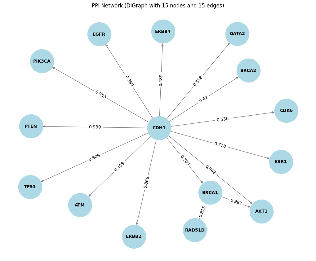
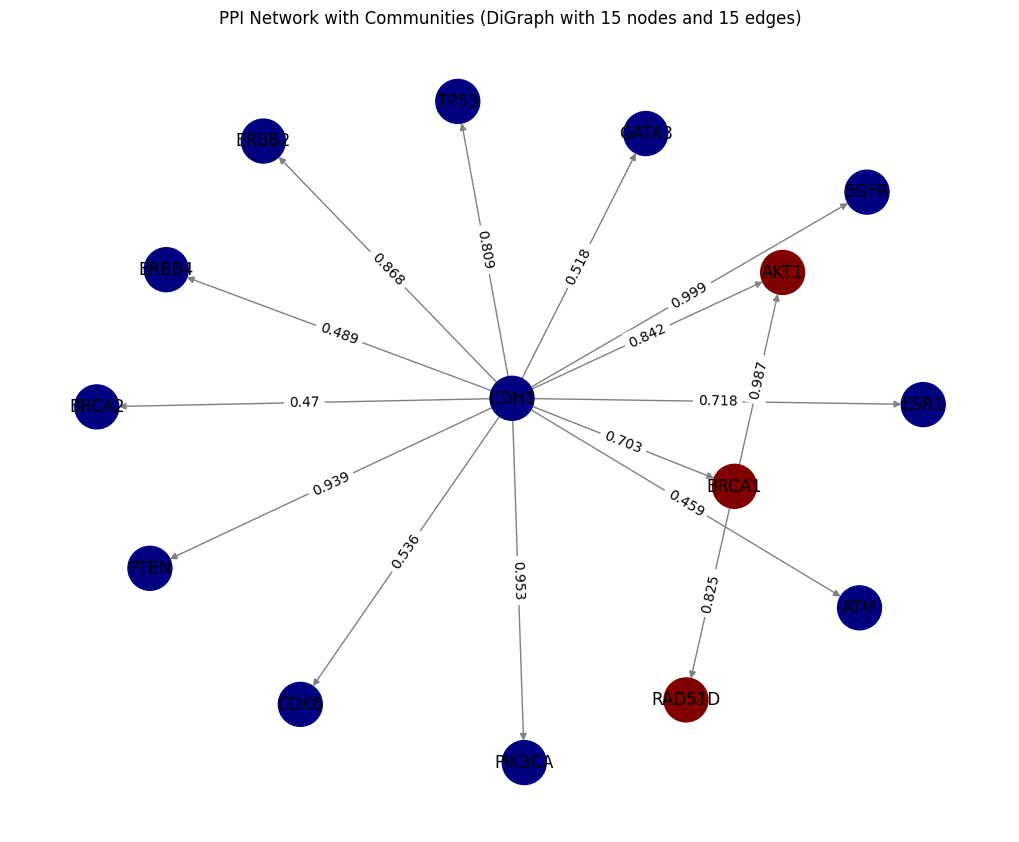
- In the STRING directed Graph the arrows indicate the direction of relationships from
preferredName_AtopreferredName_B. The weight represents as thescorevalue for each edge
Tut_STRING_DiGraph = plot_DiGraph(tut_STRING_df,'preferredName_A', 'preferredName_B', 'score')
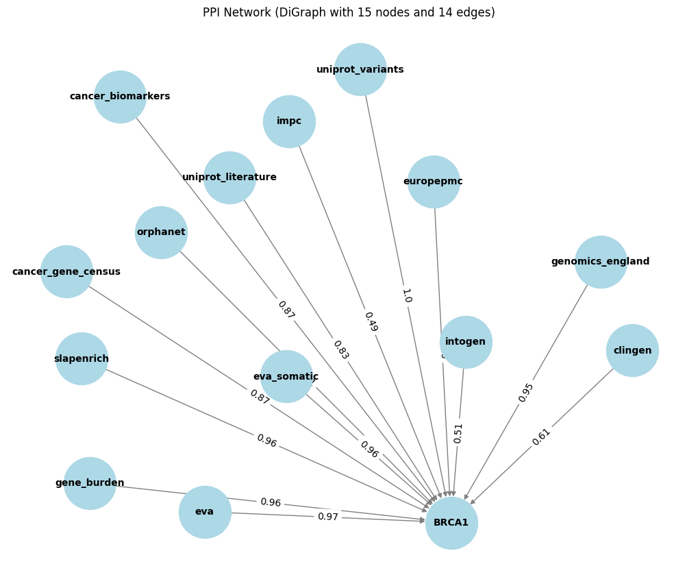
# similary we can see the directed graph in the open target dataset
tut_open_target_df = open_target_df.copy()
# Filter the df to include only rows with the a specific gene symbol
tut_open_target_df = tut_open_target_df[tut_open_target_df['approvedSymbol'] == 'BRCA1']
# Round the 'score' column to 2 decimal places
tut_open_target_df['datasourceScores_score'] = tut_open_target_df['datasourceScores_score'].round(2)

# plot the directed graph
Tut_open_target_DiGraph = plot_DiGraph(tut_open_target_df, 'datasourceScores_id', 'approvedSymbol', 'datasourceScores_score')
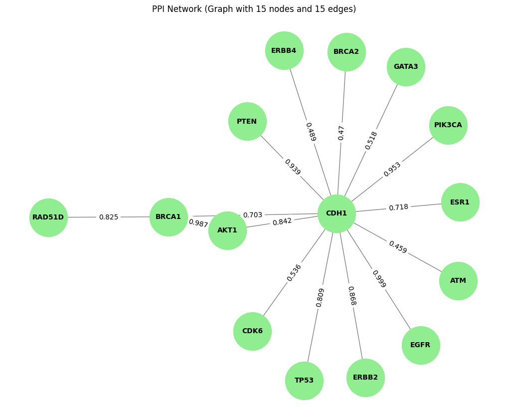
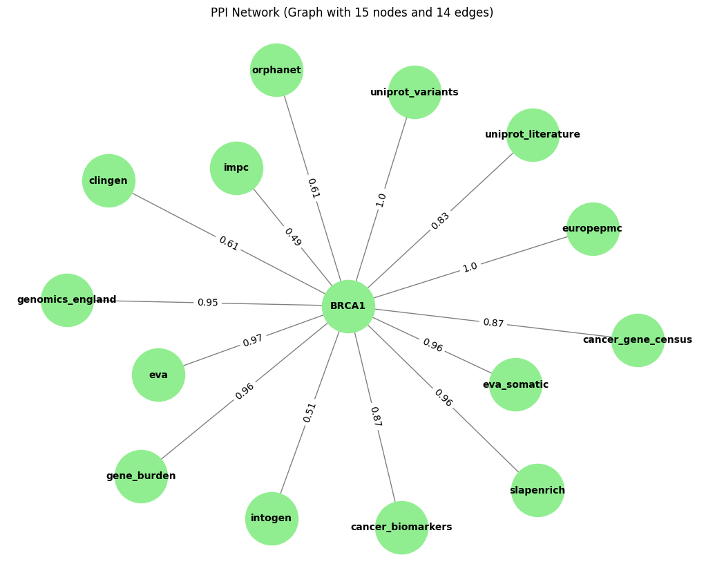
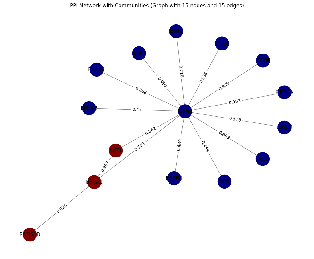
Creating Undirected Graphs
- In the undirected Graph, there are no arrows because edges are bidirectional. The weight (scores) remains unchanged, and edge direction is not considered
def plot_Graph(
        df: pd.DataFrame,
        source_col: str,
        target_col: str,
        edge_attr_col: str,
        figsize: tuple = (10, 8)
) -> None:
    """
    Create and plot a undirected graph from the given df
    """
    # create a undirected graph from the DataFrame
    G = nx.from_pandas_edgelist(
        df,
        source=source_col,
        target=target_col,
        edge_attr=edge_attr_col,
        create_using=nx.Graph()  # notice the undirect Graph
    )

    # plot the undirected graph
    plt.figure(figsize=figsize)
    pos = nx.spring_layout(G)
    nx.draw(
        G,
        pos,
        with_labels=True,
        node_color='lightgreen',
        edge_color='gray',
        node_size=3000,
        font_size=10,
        font_weight='bold',
        arrows=True
    )

    edge_labels = nx.get_edge_attributes(G, edge_attr_col)
    nx.draw_networkx_edge_labels(G, pos, edge_labels=edge_labels)
    plt.title(f'PPI Network ({G})')
    plt.show()
    return G
Tut_STRING_Graph = plot_Graph(tut_STRING_df,'preferredName_A', 'preferredName_B', 'score')
Tut_open_target_Graph = plot_Graph(tut_open_target_df, 'datasourceScores_id', 'approvedSymbol', 'datasourceScores_score')
Which Graph we chose?
For a general PPI networks where interactions are typically mutual and direction is not that important, we use an undirected graph, as it’s the common choice for most PPI studies. However, if we ever need to direct these graphs, we now know where to look
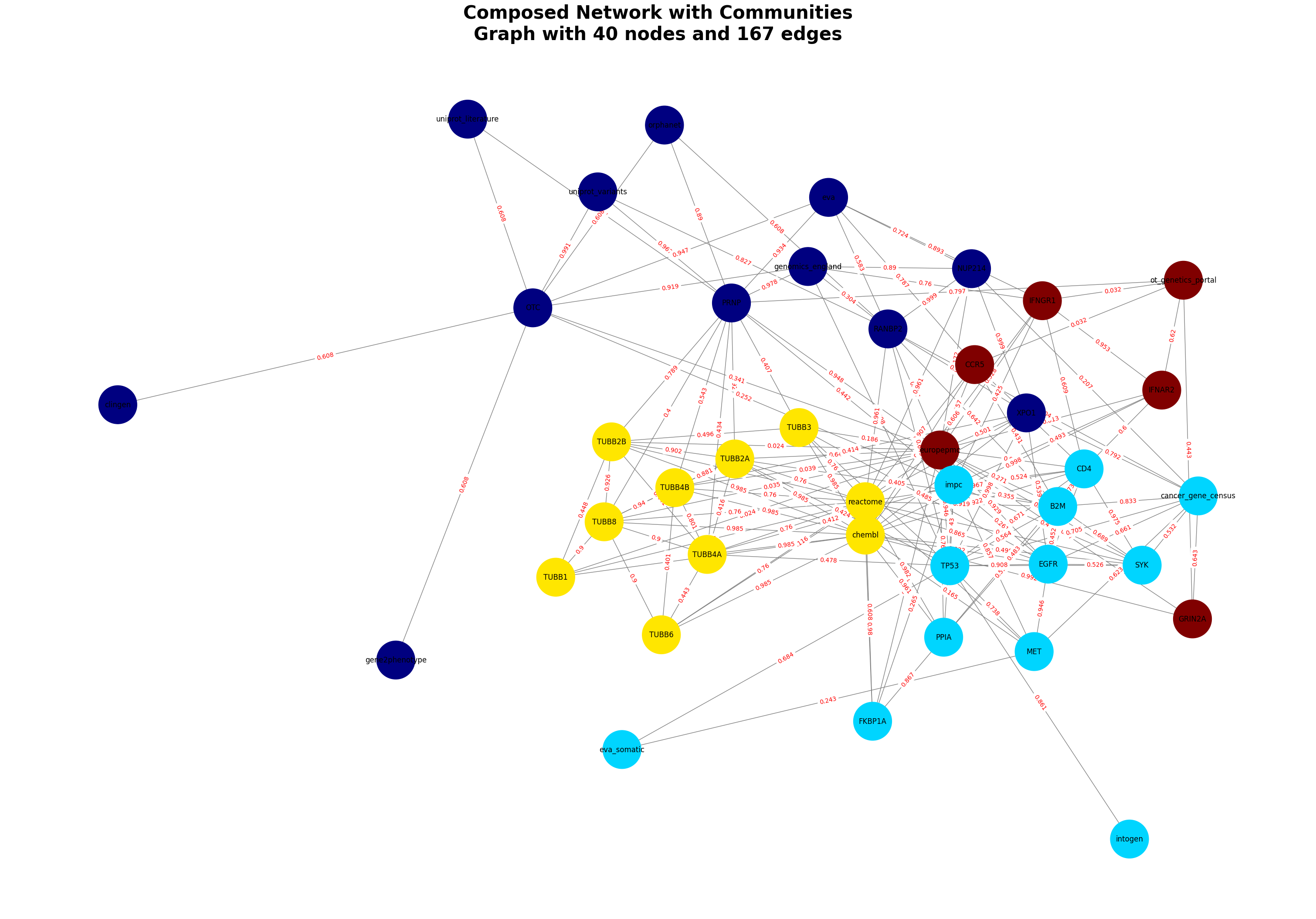
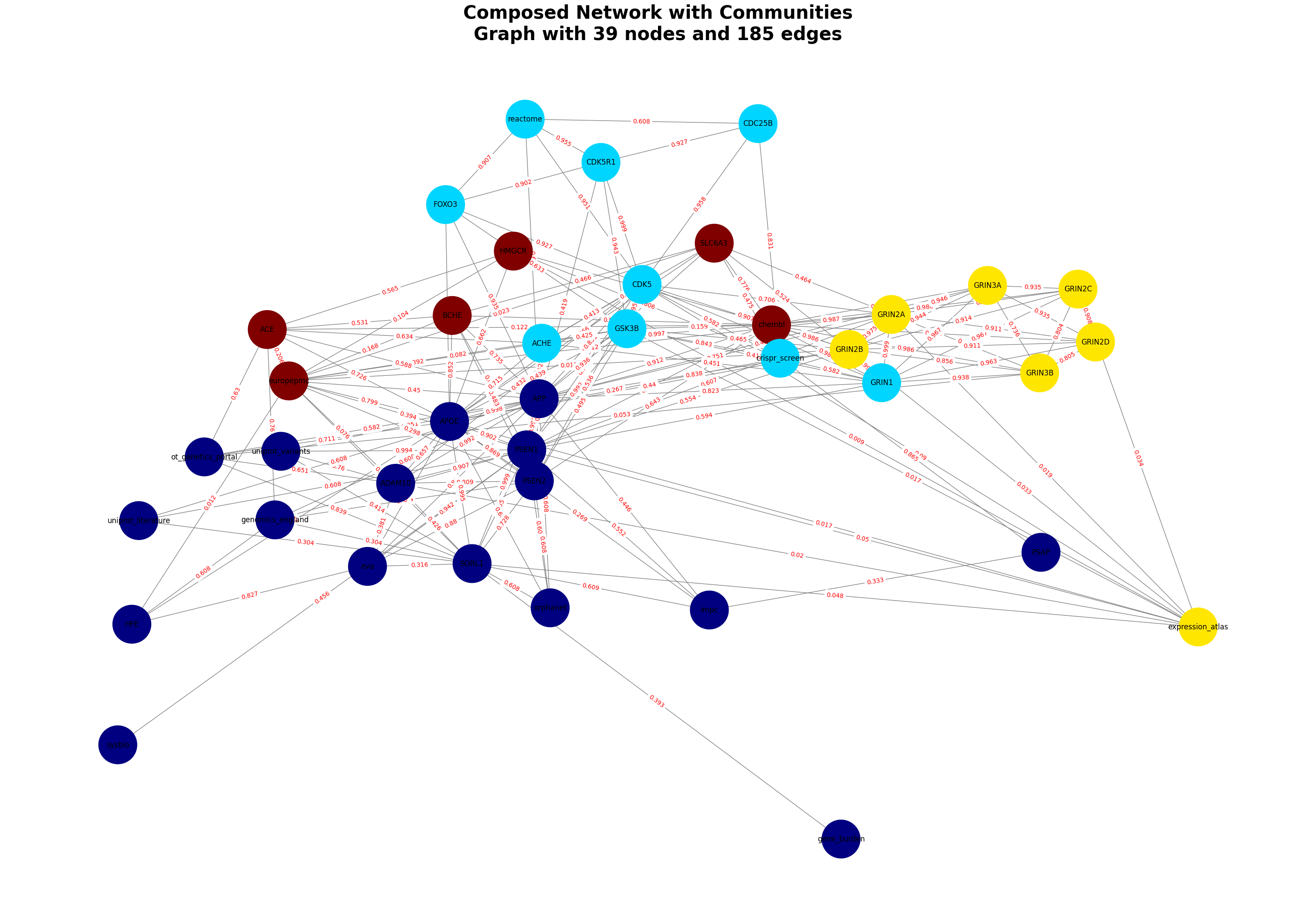
Detecting Communities in Graphs
- Community detection identifies groups of nodes in a graph that are more connected to each other than to the rest of the network
- Each community is assigned a distinct color, so nodes in the same community (cluster) share the same color
- Colors help to easily visualize and distinguish different communities (clusters) within the network
def plot_community_detection(graph, edge_attr_col: str, figsize: tuple = (10, 8))-> None:
    """
    plots graph with community detection
    """
    communities = community.greedy_modularity_communities(graph)

    # Color nodes by community
    colors = [0] * graph.number_of_nodes()
    for i, comm in enumerate(communities):
        for node in comm:
            colors[list(graph.nodes()).index(node)] = i

    # Plotting
    plt.figure(figsize=figsize)
    pos = nx.spring_layout(graph)
    nx.draw(
        graph,
        pos, with_labels=True,
        node_color=colors,
        cmap=plt.cm.jet, node_size=1000, edge_color='gray', arrows=True
    )
    edge_labels = nx.get_edge_attributes(graph, edge_attr_col)
    nx.draw_networkx_edge_labels(graph, pos, edge_labels=edge_labels)
    plt.title(f'PPI Network with Communities ({graph})')
    plt.show()
plot_community_detection(Tut_STRING_DiGraph, edge_attr_col ='score')
plot_community_detection(Tut_STRING_Graph, edge_attr_col = 'score')
Disease-Specific Graph Construction
Building Breast Cancer Interaction Networks
we already fetched the breast cancer dataset in this section
# breast cancer dataset
open_target_df
| datasourceScores_id | datasourceScores_score | score | id | approvedSymbol | |
|---|---|---|---|---|---|
| 0 | uniprot_variants | 0.996781 | 0.924615 | ENSG00000139618 | BRCA2 |
| 1 | gene_burden | 0.981427 | 0.924615 | ENSG00000139618 | BRCA2 |
| 2 | genomics_england | 0.977902 | 0.924615 | ENSG00000139618 | BRCA2 |
| 3 | eva | 0.969933 | 0.924615 | ENSG00000139618 | BRCA2 |
| 4 | eva_somatic | 0.948894 | 0.924615 | ENSG00000139618 | BRCA2 |
| ... | ... | ... | ... | ... | ... |
| 209 | chembl | 0.976998 | 0.740814 | ENSG00000177084 | POLE |
| 210 | cancer_gene_census | 0.705094 | 0.740814 | ENSG00000177084 | POLE |
| 211 | slapenrich | 0.833427 | 0.740814 | ENSG00000177084 | POLE |
| 212 | eva | 0.278570 | 0.740814 | ENSG00000177084 | POLE |
| 213 | europepmc | 0.199886 | 0.740814 | ENSG00000177084 | POLE |
214 rows × 5 columns
open_target_df['datasourceScores_score'] = open_target_df['datasourceScores_score'].round(3)
STRING_df
| stringId_A | stringId_B | preferredName_A | preferredName_B | ncbiTaxonId | score | nscore | fscore | pscore | ascore | escore | dscore | tscore | |
|---|---|---|---|---|---|---|---|---|---|---|---|---|---|
| 0 | 9606.ENSP00000257566 | 9606.ENSP00000269305 | TBX3 | TP53 | 9606 | 0.400 | 0.0 | 0 | 0.0 | 0.000 | 0.000 | 0.0 | 0.400 |
| 1 | 9606.ENSP00000257566 | 9606.ENSP00000269305 | TBX3 | TP53 | 9606 | 0.400 | 0.0 | 0 | 0.0 | 0.000 | 0.000 | 0.0 | 0.400 |
| 2 | 9606.ENSP00000257566 | 9606.ENSP00000261769 | TBX3 | CDH1 | 9606 | 0.425 | 0.0 | 0 | 0.0 | 0.062 | 0.000 | 0.0 | 0.413 |
| 3 | 9606.ENSP00000257566 | 9606.ENSP00000261769 | TBX3 | CDH1 | 9606 | 0.425 | 0.0 | 0 | 0.0 | 0.062 | 0.000 | 0.0 | 0.413 |
| 4 | 9606.ENSP00000257566 | 9606.ENSP00000382423 | TBX3 | MAP3K1 | 9606 | 0.468 | 0.0 | 0 | 0.0 | 0.000 | 0.065 | 0.0 | 0.455 |
| ... | ... | ... | ... | ... | ... | ... | ... | ... | ... | ... | ... | ... | ... |
| 391 | 9606.ENSP00000406046 | 9606.ENSP00000418960 | POLD1 | BRCA1 | 9606 | 0.978 | 0.0 | 0 | 0.0 | 0.198 | 0.391 | 0.9 | 0.613 |
| 392 | 9606.ENSP00000418960 | 9606.ENSP00000466399 | BRCA1 | RAD51D | 9606 | 0.825 | 0.0 | 0 | 0.0 | 0.126 | 0.095 | 0.0 | 0.797 |
| 393 | 9606.ENSP00000418960 | 9606.ENSP00000466399 | BRCA1 | RAD51D | 9606 | 0.825 | 0.0 | 0 | 0.0 | 0.126 | 0.095 | 0.0 | 0.797 |
| 394 | 9606.ENSP00000418960 | 9606.ENSP00000451828 | BRCA1 | AKT1 | 9606 | 0.987 | 0.0 | 0 | 0.0 | 0.000 | 0.835 | 0.8 | 0.657 |
| 395 | 9606.ENSP00000418960 | 9606.ENSP00000451828 | BRCA1 | AKT1 | 9606 | 0.987 | 0.0 | 0 | 0.0 | 0.000 | 0.835 | 0.8 | 0.657 |
396 rows × 13 columns
Method 1: Using from_pandas_edgelist and compose
# create a graph for open target data
G = nx.from_pandas_edgelist(
    open_target_df,
    source='datasourceScores_id',
    target='approvedSymbol',
    edge_attr='datasourceScores_score',
    # edge_attr=['datasourceScores_score', 'score'],
    create_using=nx.Graph()
)

for u, v, data in G.edges(data=True):
    data['weight'] = data.pop('datasourceScores_score')  # Assign weight
    data['type'] = 'disease-gene'
# Create a graph for the STRING dataframe
H = nx.from_pandas_edgelist(
    STRING_df,
    source='preferredName_A',
    target='preferredName_B',
    edge_attr='score',
    # edge_attr=['score', 'nscore', 'fscore', 'pscore', 'ascore', 'escore', 'dscore', 'tscore'],
    create_using=nx.Graph()
)

for u, v, data in H.edges(data=True):
    data['weight'] = data.pop('score') # Assign weight
    data['type'] = 'protein-protein'
# Merge the two graphs
G_composed = nx.compose(G, H)
plt.figure(figsize=(30, 20))

pos = nx.spring_layout(G_composed, seed=42, k=0.7, iterations=90)  # Adjust 'k' and 'iterations' for better spacing

# Draw nodes with labels
nx.draw_networkx(G_composed, pos, with_labels=True, node_size=3000, font_size=10, font_weight='bold', edge_color='gray')
edge_labels = nx.get_edge_attributes(G_composed, 'weight')
nx.draw_networkx_edge_labels(G_composed, pos, edge_labels, font_color='red')

plt.axis('off')
plt.title(f"Breast Cancer Disease Associated Genes", fontsize=30, fontweight='bold')
plt.tight_layout()
# os.makedirs('assets', exist_ok=True)
# plt.savefig(f'assets/{disease_id}_{G_composed}.png')
plt.show()
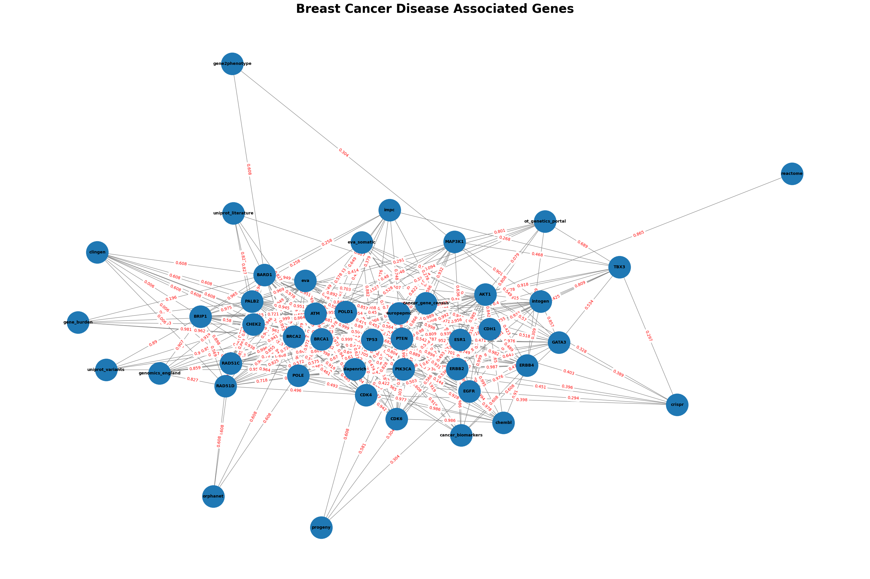
these edge attributes are preserved, and they can be accessed later using nx.get_edge_attributes with the specific attribute name score or datasourceScores_score
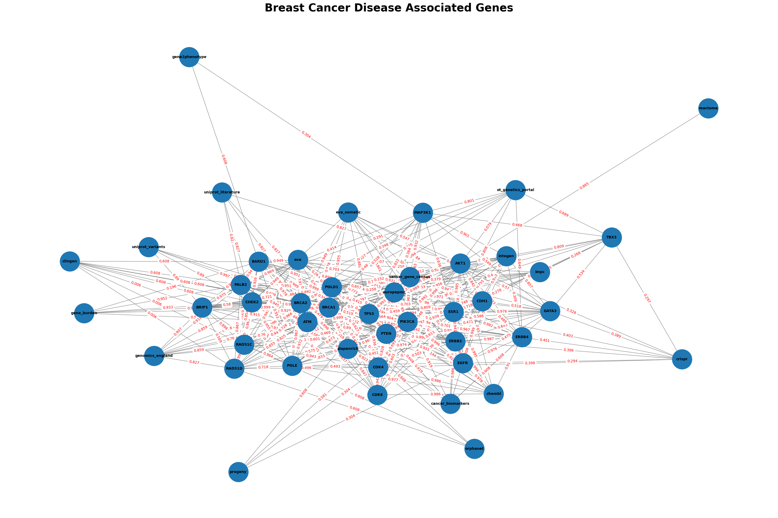
Method 2: Manually Adding Edges with add_edge and compose
G2 = nx.Graph()
for _, row in open_target_df.iterrows():
    G2.add_edge(row['datasourceScores_id'],
               row['approvedSymbol'],
               weight=row['datasourceScores_score'],
               type='disease-gene')

H2 = nx.Graph()
for _, row in STRING_df.iterrows():
    H2.add_edge(row['preferredName_A'],
               row['preferredName_B'],
               weight=row['score'],
               type='protein-protein')
# Merge the two graphs
G_composed2 = nx.compose(G2, H2)
plt.figure(figsize=(30, 20))

pos = nx.spring_layout(G_composed2, seed=42, k=0.9, iterations=100)  # Adjust 'k' and 'iterations' for better spacing


# Draw nodes with labels
nx.draw_networkx(G_composed2, pos, with_labels=True, node_size=3000, font_size=10, font_weight='bold', edge_color='gray')

edge_labels = nx.get_edge_attributes(G_composed2, 'weight')
nx.draw_networkx_edge_labels(G_composed2, pos, edge_labels, font_color='red')

plt.axis('off')
plt.title(f"Breast Cancer Disease Associated Genes", fontsize=30, fontweight='bold')
plt.tight_layout()
# plt.savefig(f'assets/{disease_id}.png')
plt.show()
Comparing Node Connections Across Methods
def get_node_edges(graph, node, edge_type=None):
    """
    Returns edges connected to specified nodes in a graph
    optionally filtered by edge type
    """
    edge_types = ['disease-gene', 'protein-protein']
    if edge_type is not None and edge_type not in edge_types:
        raise ValueError(f"Invalid edge type. Must be one of {edge_types}.")
    edges = list(graph.edges(node, data=True))
    if edge_type:
        edges = [edge for edge in edges if edge[2].get('type') == edge_type]
    return edges

def edge_to_tuple(edge):
    """Convert edge to a tuple with dictionaries as frozensets"""
    u, v, attr = edge
    attr_frozenset = frozenset(attr.items())
    return (u, v, attr_frozenset)
node = 'ERBB4'
edges_composed = get_node_edges(G_composed, node, edge_type='protein-protein')
edges_composed2 = get_node_edges(G_composed2, node, edge_type='protein-protein')

print(f"Edges connected to {node} in {G_composed}:")
for edge in edges_composed[:5]:
    print(edge)

print(f"\nEdges connected to {node} in {G_composed2}:")
for edge in edges_composed2[:5]:
    print(edge)

edges_composed_set = set(edge_to_tuple(edge) for edge in edges_composed)
edges_composed2_set = set(edge_to_tuple(edge) for edge in edges_composed2)
if edges_composed_set == edges_composed2_set:
    print("\nThe sets of edges are identical.")
Edges connected to ERBB4 in Graph with 45 nodes and 412 edges:
('ERBB4', 'TP53', {'weight': 0.701, 'type': 'protein-protein'})
('ERBB4', 'CDH1', {'weight': 0.489, 'type': 'protein-protein'})
('ERBB4', 'ESR1', {'weight': 0.982, 'type': 'protein-protein'})
('ERBB4', 'ERBB2', {'weight': 0.987, 'type': 'protein-protein'})
('ERBB4', 'AKT1', {'weight': 0.423, 'type': 'protein-protein'})

The sets of edges are identical.
Integrating Graphs and Class Definitions
import sys
sys.path.append('../src')
from graph_composer import GraphComposer
Generating Graphs for Infectious Diseases
The dataset for the Infectious Disease is identified by EFO_0005741
disease_id = "EFO_0005741"
disease_name="Infectious"
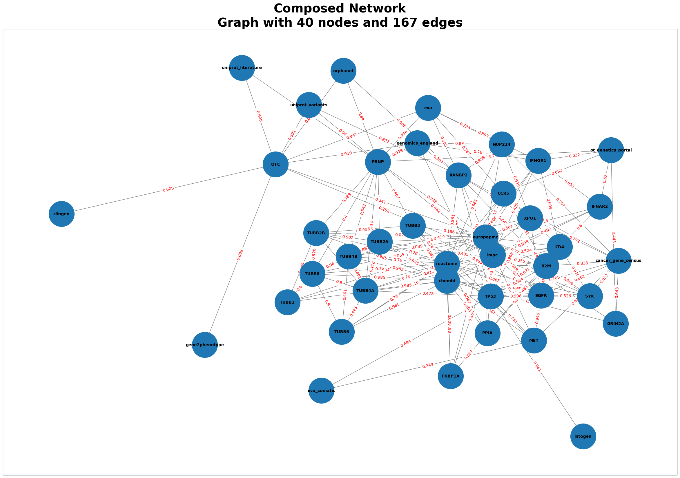
Infectious = GraphComposer(disease_id, disease_name)
Infectious.process_all(plot=True)
# Accessing the features, and genes
features = Infectious.features
df = Infectious.open_target_df
gene = Infectious.gene_symbols

score = get_feature_score(df, gene_symbol = 'PRNP', feature_key='orphanet')
orphanet score for PRNP: 0.89
merged_df = Infectious.get_merged_dataframe()
print(merged_df.describe)
print(merged_df.info())
<bound method NDFrame.describe of                source  target  weight             type
0    genomics_england    PRNP   0.978     disease-gene
1    genomics_england     OTC   0.919     disease-gene
2    genomics_england  RANBP2   0.304     disease-gene
3    genomics_england  NUP214   0.890     disease-gene
4    genomics_england    TP53   0.608     disease-gene
..                ...     ...     ...              ...
162              XPO1    EGFR   0.539  protein-protein
163              EGFR     B2M   0.452  protein-protein
164              EGFR     SYK   0.526  protein-protein
165              EGFR     MET   0.946  protein-protein
166               SYK     B2M   0.689  protein-protein

[167 rows x 4 columns]>
<class 'pandas.core.frame.DataFrame'>
RangeIndex: 167 entries, 0 to 166
Data columns (total 4 columns):
 #   Column  Non-Null Count  Dtype
---  ------  --------------  -----
 0   source  167 non-null    object
 1   target  167 non-null    object
 2   weight  167 non-null    float64
 3   type    167 non-null    object
dtypes: float64(1), object(3)
memory usage: 5.3+ KB
None
merged_df.head()
| source | target | weight | type | |
|---|---|---|---|---|
| 0 | genomics_england | PRNP | 0.978 | disease-gene |
| 1 | genomics_england | OTC | 0.919 | disease-gene |
| 2 | genomics_england | RANBP2 | 0.304 | disease-gene |
| 3 | genomics_england | NUP214 | 0.890 | disease-gene |
| 4 | genomics_england | TP53 | 0.608 | disease-gene |
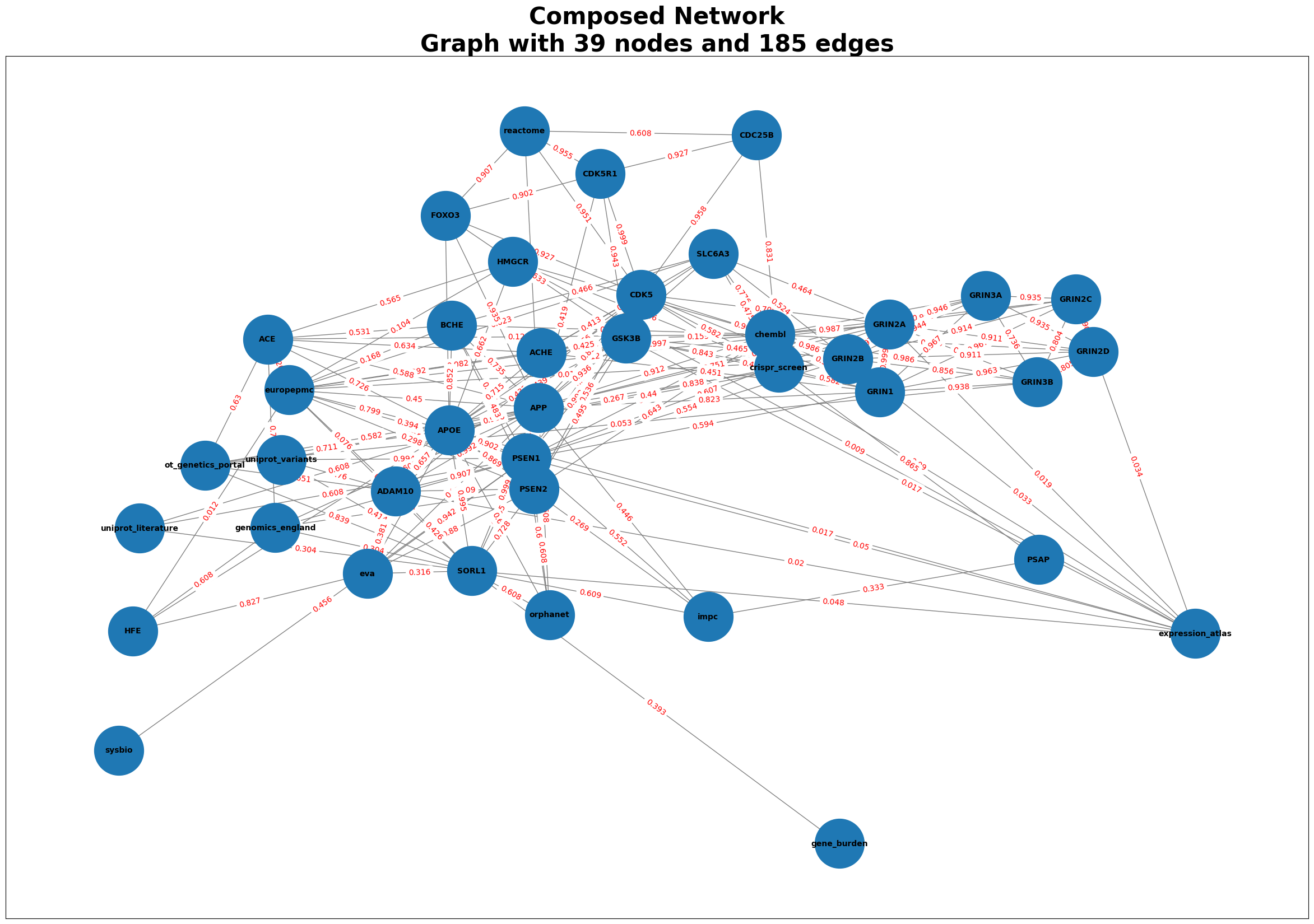
Generating Graphs for Alzheimer’s Disease
The dataset for the Alzheimer Disease is identified by MONDO_0004975
disease_id = "MONDO_0004975"
Alzheimer = GraphComposer(disease_id, disease_name="Alzheimer")
Alzheimer.process_all(plot=True)
# Accessing the merged_df
merged_df2 = Alzheimer.get_merged_dataframe()
merged_df2.head()
| source | target | weight | type | |
|---|---|---|---|---|
| 0 | uniprot_variants | PSEN1 | 0.994 | disease-gene |
| 1 | uniprot_variants | APP | 0.951 | disease-gene |
| 2 | uniprot_variants | SORL1 | 0.414 | disease-gene |
| 3 | uniprot_variants | ADAM10 | 0.760 | disease-gene |
| 4 | PSEN1 | genomics_england | 0.955 | disease-gene |